Machine Learning - Polynomial Regression

Polynomial Regression

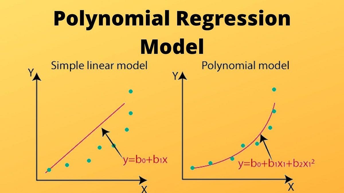
If your data points clearly will not fit a linear regression (a straight line through all data points), it might be ideal for polynomial regression.

Non-linear Relationships: Polynomial regression is used when the relationship between the independent variable (input) and dependent variable (output) is non-linear. Unlike linear regression which fits a straight line, it fits a polynomial equation to capture the curve in the data.

Better Fit for Curved Data: When a researcher hypothesizes a curvilinear relationship, polynomial terms are added to the model. A linear model often results in residuals with noticeable patterns which shows a poor fit. It can capture these non-linear patterns effectively.

Flexibility and Complexity: It does not assume all independent variables are independent. By introducing higher-degree terms, it allows for more flexibility and can model more complex, curvilinear relationships between variables

Polynomial regression, like linear regression, uses the relationship between the variables x and y to find the best way to draw a line through the data points.

How Does it Work?

Python has methods for finding a relationship between data-points and to draw a line of polynomial regression. We will show you how to use these methods instead of going through the mathematic formula.

In the example below, we have registered 18 cars as they were passing a certain tollbooth. The x-axis represents the hours of the day and the y-axis represents the speed.

Example: Start by drawing a scatter plot

import matplotlib.pyplot as plt

x = [1,2,3,5,6,7,8,9,10,12,13,14,15,16,18,19,21,22]
y = [100,90,80,60,60,55,60,65,70,70,75,76,78,79,90,99,99,100]

plt.scatter(x, y)
plt.show()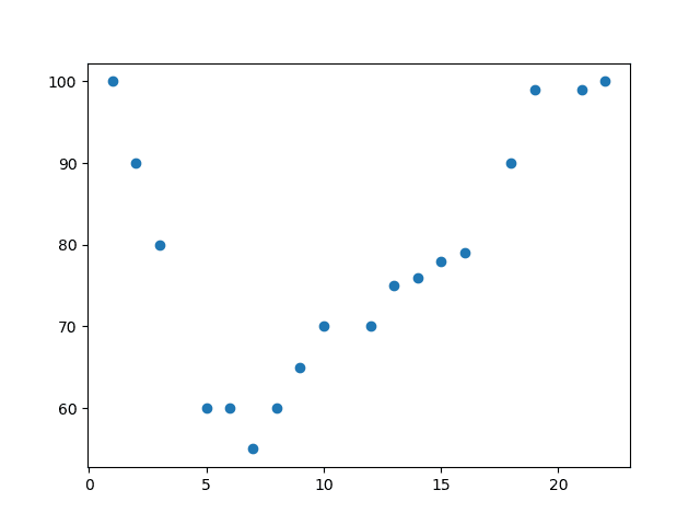

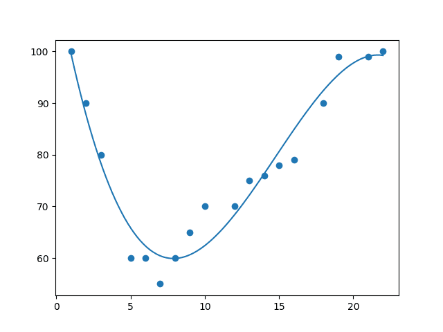
Example: Import numpy and matplotlib then draw the line

import numpy
import matplotlib.pyplot as plt

x = [1,2,3,5,6,7,8,9,10,12,13,14,15,16,18,19,21,22]
y = [100,90,80,60,60,55,60,65,70,70,75,76,78,79,90,99,99,100]

mymodel = numpy.poly1d(numpy.polyfit(x, y, 3))
myline = numpy.linspace(1, 22, 100)

plt.scatter(x, y)
plt.plot(myline, mymodel(myline))
plt.show()

Example Explained

Import the modules you need:

import numpy
import matplotlib.pyplot as plt

Create the arrays that represent the values of the x and y axis:

x = [1,2,3,5,6,7,8,9,10,12,13,14,15,16,18,19,21,22]
y = [100,90,80,60,60,55,60,65,70,70,75,76,78,79,90,99,99,100]

NumPy has a method that lets us make a polynomial model:

mymodel = numpy.poly1d(numpy.polyfit(x, y, 3))

Then specify how the line will display, we start at position 1, and end at position 22:

myline = numpy.linspace(1, 22, 100)

Draw the original scatter plot:

plt.scatter(x, y)

Draw the line of polynomial regression:

plt.plot(myline, mymodel(myline))

Display the diagram:

plt.show()

R-Squared

It is important to know how well the relationship between the values of the x- and y-axis is, if there are no relationship the polynomial regression can not be used to predict anything.

The relationship is measured with a value called the r-squared.

The r-squared value ranges from 0 to 1, where 0 means no relationship, and 1 means 100% related.

import numpy
from sklearn.metrics import r2_score

x = [1,2,3,5,6,7,8,9,10,12,13,14,15,16,18,19,21,22]
y = [100,90,80,60,60,55,60,65,70,70,75,76,78,79,90,99,99,100]

mymodel = numpy.poly1d(numpy.polyfit(x, y, 3))

print(r2_score(y, mymodel(x)))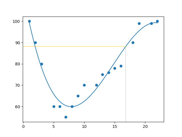

Note: The result 0.94 shows that there is a very good relationship, and we can use polynomial regression in future predictions.

Predict Future Values

Now we can use the information we have gathered to predict future values.

Example: Let us try to predict the speed of a car that passes the tollbooth at around 17:00:

import numpy
from sklearn.metrics import r2_score

x = [1,2,3,5,6,7,8,9,10,12,13,14,15,16,18,19,21,22]
y = [100,90,80,60,60,55,60,65,70,70,75,76,78,79,90,99,99,100]

mymodel = numpy.poly1d(numpy.polyfit(x, y, 3))

speed = mymodel(17)
print(speed)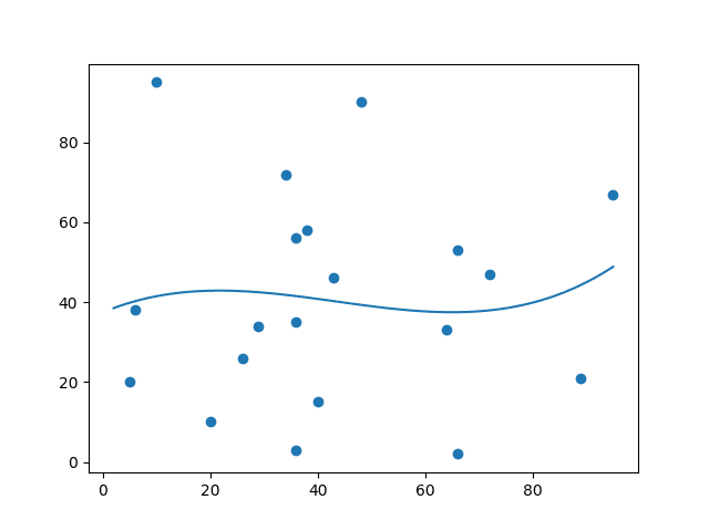

The example predicted a speed to be 88.87.

Bad Fit?

Let us create an example where polynomial regression would not be the best method to predict future values.

import numpy
import matplotlib.pyplot as plt

x = [89,43,36,36,95,10,66,34,38,20,26,29,48,64,6,5,36,66,72,40]
y = [21,46,3,35,67,95,53,72,58,10,26,34,90,33,38,20,56,2,47,15]

mymodel = numpy.poly1d(numpy.polyfit(x, y, 3))
myline = numpy.linspace(2, 95, 100)

plt.scatter(x, y)
plt.plot(myline, mymodel(myline))
plt.show()

And the r-squared value?

import numpy
from sklearn.metrics import r2_score

x = [89,43,36,36,95,10,66,34,38,20,26,29,48,64,6,5,36,66,72,40]
y = [21,46,3,35,67,95,53,72,58,10,26,34,90,33,38,20,56,2,47,15]

mymodel = numpy.poly1d(numpy.polyfit(x, y, 3))

print(r2_score(y, mymodel(x)))

The result: 0.00995 indicates a very bad relationship, and tells us that this data set is not suitable for polynomial regression.