
Machine Learning - Normal Data Distribution
Normal Data Distribution
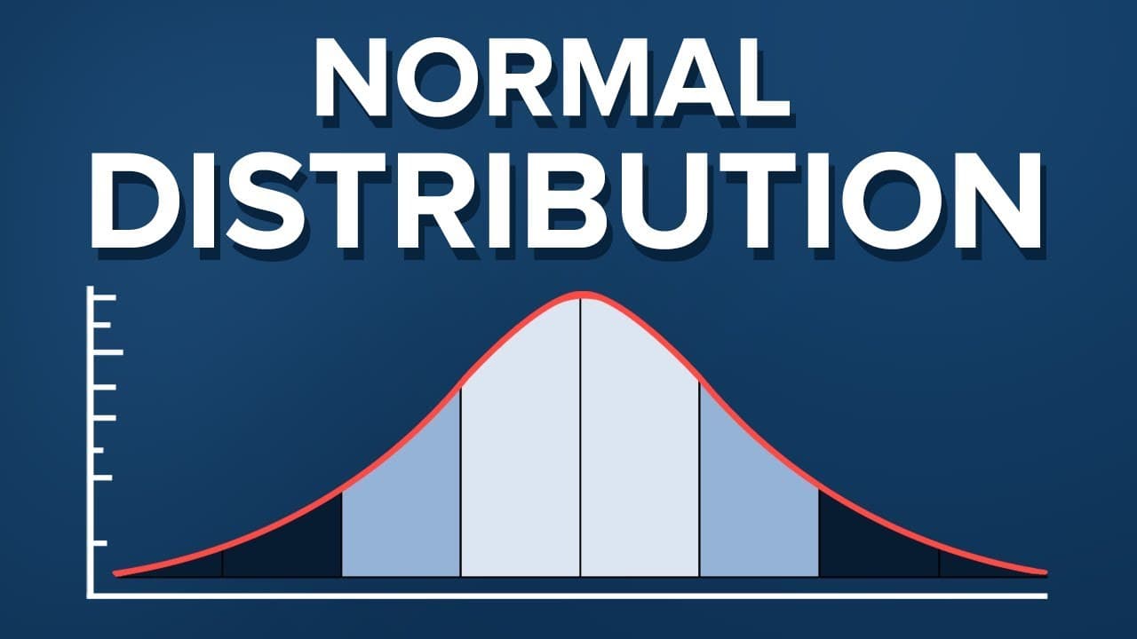
The Normal Distribution (also called the Gaussian or Bell-shaped Distribution) is one of the most commonly used probability distributions in statistics. It is symmetric around the mean and forms the characteristic bell-shaped curve

In the previous chapter we learned how to create a completely random array, of a given size, and between two given values.
In this chapter we will learn how to create an array where the values are concentrated around a given value.
In probability theory this kind of data distribution is known as the normal data distribution, or the Gaussian data distribution, after the mathematician Carl Friedrich Gauss who came up with the formula of this data distribution.
The Normal Distribution (also called the Gaussian or Bell-shaped Distribution) is one of the most commonly used probability distributions in statistics. It is symmetric around the mean and forms the characteristic bell-shaped curve. It plays an essential role in statistics, especially in the Central Limit Theorem (CLT). Most values cluster near the mean and the probability decreases as we move away from it.
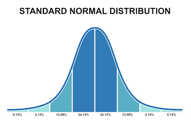
It can be observed in the above image that the distribution is symmetric about its center which is the mean (0 in this case). This makes the probability of events at equal deviations from the mean equally probable. The density is highly centered around the mean which translates to lower probabilities for values away from the mean.
Example
A typical normal data distribution:
import numpy
import matplotlib.pyplot as plt

x = numpy.random.normal(5.0, 1.0, 100000)

plt.hist(x, 100)
plt.show()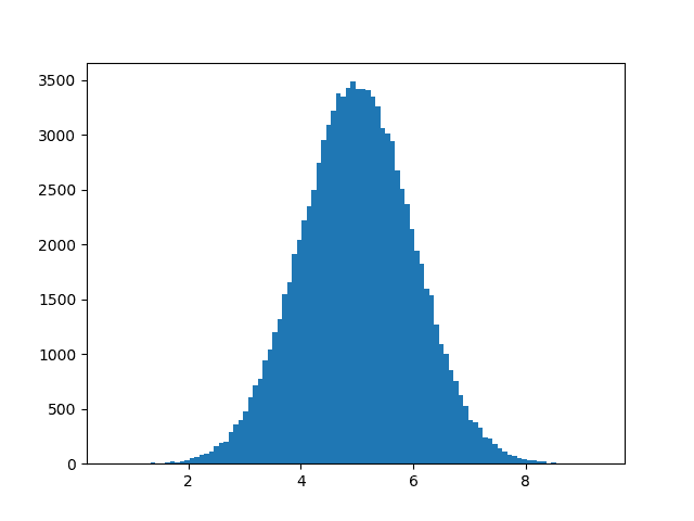
Note: A normal distribution graph is also known as the bell curve because of it's characteristic shape of a bell.
Histogram Explained
We use the array from the numpy.random.normal() method, with 100000 values, to draw a histogram with 100 bars.
We specify that the mean value is 5.0, and the standard deviation is 1.0.
Meaning that the values should be concentrated around 5.0, and rarely further away than 1.0 from the mean.
And as you can see from the histogram, most values are between 4.0 and 6.0, with a top at approximately 5.0.