Machine Learning - Data Distribution

Data Distribution

A statistical data distribution is a function that shows the possible values of a variable and how frequently they occur. It provides a mathematical description of the data’s behavior which indicate where most data points are concentrated and how they are spread out. Distributions can be represented in various forms such as probability density functions for continuous data or probability mass functions for discrete data.

Earlier in this tutorial we have worked with very small amounts of data in our examples, just to understand the different concepts.

In the real world, the data sets are much bigger, but it can be difficult to gather real world data, at least at an early stage of a project.

A statistical data distribution is a function that shows the possible values of a variable and how frequently they occur. It provides a mathematical description of the data’s behavior which indicate where most data points are concentrated and how they are spread out. Distributions can be represented in various forms such as probability density functions for continuous data or probability mass functions for discrete data.

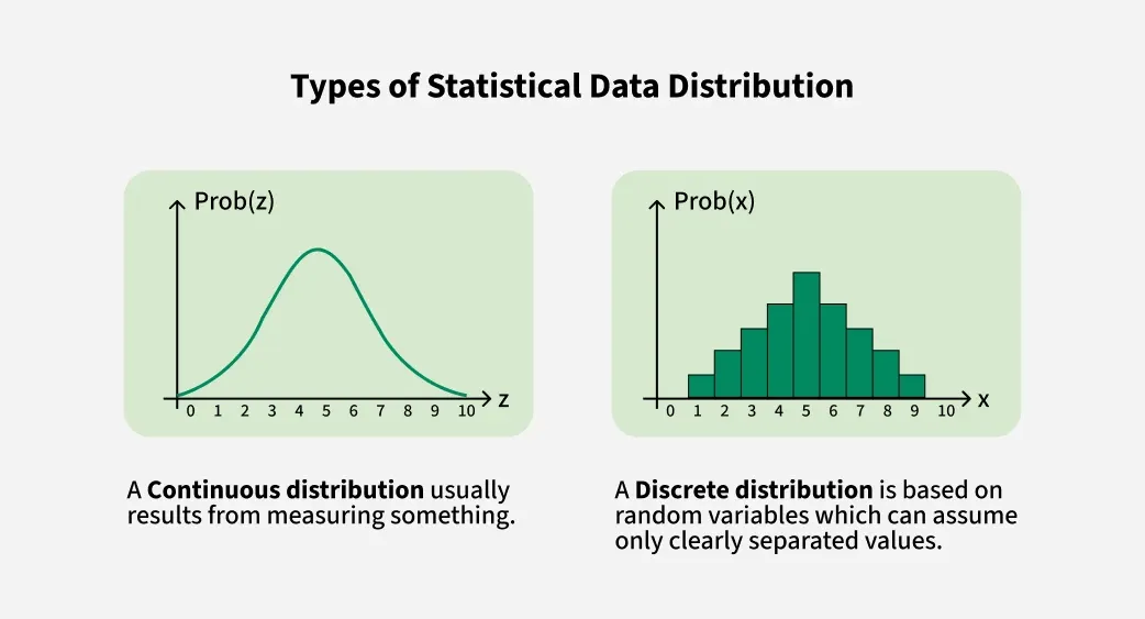
Discrete Distributions:

A discrete distribution is used when the data can take only certain separate values. These values are countable like 1, 2, 3 and so on. You can’t have values in between like 1.5 or 2.7.

For example the number of books on a shelf or the number of students in a class is discrete. Some common types of discrete distributions include the Binomial distribution, Poisson distribution and more

Continuous Distributions:

A continuous distribution is used when the data can take any value within a range including fractions and decimals. This is used for things you can measure like height, weight, temperature or time.

For example someone can be 165.3 cm tall or a race can take 12.75 seconds. Common types of continuous distributions include the Normal distribution , Exponential distribution and more

How Can we Get Big Data Sets?

To create big data sets for testing, we use the Python module NumPy, which comes with a number of methods to create random data sets, of any size.

Example

Create an array containing 250 random floats between 0 and 5:

import numpy

x = numpy.random.uniform(0.0, 5.0, 250)

print(x)

Histogram

To visualize the data set we can draw a histogram with the data we collected.

We will use the Python module Matplotlib to draw a histogram.

Example

Draw a histogram:

import numpy
import matplotlib.pyplot as plt

x = numpy.random.uniform(0.0, 5.0, 250)

plt.hist(x, 5)
plt.show()

Result:

Histogram Explained

We use the array from the example above to draw a histogram with 5 bars.

The first bar represents how many values in the array are between 0 and 1.

The second bar represents how many values are between 1 and 2.

Etc.

Which gives us this result:

52 values are between 0 and 1
48 values are between 1 and 2
49 values are between 2 and 3
51 values are between 3 and 4
50 values are between 4 and 5

Note: The array values are random numbers and will not show the exact same result on your computer.

Big Data Distributions

An array containing 250 values is not considered very big, but now you know how to create a random set of values, and by changing the parameters, you can create the data set as big as you want.

Example

Create an array with 100000 random numbers, and display them using a histogram with 100 bars:

import numpy
import matplotlib.pyplot as plt

x = numpy.random.uniform(0.0, 5.0, 100000)

plt.hist(x, 100)
plt.show()